Chasing Data Using Sleuth Kit

Working on a new set of videos for O'Reilly Media -- basically updating one of the first video titles from back when it was Infinite Skills. In the process, I had to refresh my memory on a number of things. One of them was using The Sleuth Kit tools to run through a disk image to locate the contents of a file. Sure, you could just pop it open in a browser using some commercial tool but where's the fun in that? Autopsy you say? Yeah, but ultimately, Autopsy uses The Sleuth Kit tools to begin with even if you don't see it. Why not just learn what it is that Autopsy does so you can be ahead of the game? Having said that, let's step through how you might go about this.

We're going to be working with a disk image taken from a Linux system and the partition on the disk was formatted with ext4. However, the same steps will work for a Windows disk, particularly if the partition was formatted with NTFS. Since we have a disk image and not a partition image, the first thing we need to do is determine where the partition actually starts. In order to do that, we are going to use the program mmls, which lists all of the partitions in a disk or disk image. We could also use fdisk -l to do essentially the same thing.

What we discover here is that the partition we are looking for starts at byte 2048. The other Sleuth Kit tools we will be using will need to be told what offset to start at because they are really looking for the start of the partition in order to parse the data structures that begin there. Once we know where the partition starts, we can get a list of the files that are in the partition. For this, I'm just going to get a list of active files and not worry about doing a recursive listing down through all the directories (adding a -r). We also aren't going to deleted files (adding a -d). For our purposes, it doesn't much matter whether we have those or not. We are going to use fls and we need to add a -o 2048 to indicate that the offset to where the partition starts is 2048 bytes.

We now have a listing of the small number of files that are in the root directory of this partition. What we get from this listing is whether the entry is a directory (d/d) or a regular file (r/r). The second column is the inode where the metadata for the file is located. The metadata for the file not only includes date information but also, more importantly, the data blocks that belong to the file. Those data blocks are where can get access to the contents of the file. In order to get the data blocks, we are going to use the program istat. This will give us all of the information that the inode has related to the file. Keep in mind that while you think about the file in the context of the filename, on a UFS-based system (ext inherits a lot from UFS, the UNIX File System that goes back to the 70s and 80s with BSD, the Berkeley Systems Distribution), a file is just a collection of related data blocks. We could have multiple filenames that all point to the same "file" on the disk.

Running istat, we provide the offset to the start of the partition, just as we did with fls. Additionally, we provide the image that we are searching and also the inode that we want to interrogate. You can see the results of this below.

Among other things, we can see that the inode has been allocated. It's not free space because it refers to a file. You can see the date and time information. You can also see the permissions that are associated with the file. Additionally, as I mentioned above, different filenames can point to the same set of data blocks (the same inode). The "num of links" entry indicates the number of filenames that point to this inode, and by extension, the data that the inode points to. This is where the "Direct Blocks" entry is important. The direct blocks tells us where to get the contents of the file. For this, we use the blkcat command.

Again, we have to provide the offset because blkcat expects to start with the beginning of the partition, as fls and istat do. We provide the image name then the block number where the data is located. This is followed in this case by the number of blocks we want to extract. By default, we only pull one but since all of the blocks for the file are consecutive, we can pull all of them at once. Beneath that, you can see the contents of the file.

While it's several steps, using mmls to get the partition start, fls to get a listing of files, istat to get the data block address and finally blkcat to extract the file contents, it does help to highlight how the filesystem is put together. Being able to follow this chain, no matter the file or the filesystem, will help with the understanding of the workings of a filesystem such that no matter what tool you are using, you know the process.

Analyzing Virtual Images

The Sleuth Kit can be used to investigate disks and disk images but the images don’t actually have to be copied from a real, physical disk. You can analyze a virtual image that you have created just as easily. The Sleuth Kit includes a number of very useful command line utilities that can be run on Windows, Linux and Mac OS X systems. For our purposes, this is being done on a Mac OS X system where the program was built using the Xcode Command Line Utilities that need to be installed before you can build The Sleuth Kit. First, let’s take a look at an image that was created on a Windows system using diskpart to create a virtual disk image and then format it. Before we do anything, we need to take a look at the partition table in the image to see where the partitions are. Without that information, we can’t go much further.

You can see from the screen capture above that we have used the mmls utility from The Sleuth Kit to get the partition table. mmls tells us that this is a DOS partition table. We aren’t restricted to the type of partition table that’s on the disk, though. Let’s take a look at another virtual disk image that was created using the Mac OS X Disk Utility program. Using mmls on that, we can see a GUID partition table.

In either case, you need to locate the partition that you want to investigate. In order to get file system statistics, we can use fsstat but we need to point fsstat at the actual partition using -o to indicate the offset within the image. In our case, we are looking at the fifth slot from mmls, which has a starting offset of 40 so that’s what we tell fsstat.

From this, we can see that it’s an HFS+ file system that was last mounted by Mac OS X and it was journaled, meaning that the operating system was keeping track of changes to the filesystem in case anything bad happened so the changes could be redone to reconstruct a clean copy of the the data, including the metadata indicating where all of the files were located. While this is all very interesting, what we probably want to get at is the actual files within the image. For that, we can use fls. This will give us a file listing of the partition. Let’s go back to the Windows image from earlier, since it had a different partition type, file system and offset. Looking at the mmls output above, the third slot is the only one that actually carries a filesystem, so that’s the one we will use. Again, we need to provide the offset to get to the actual filesystem and in this case, the offset is 128.

Once we have the list of files that were stored in the file table, which in this case is the Master File Table (MFT) from the NT File System (NTFS), we can do a bit more digging into files if we chose to. What you see here are the entries within the file table only and with the MFT, there is a lot more information to be gathered. First, we need to know where to look. Find the entry for Diskpart1.png above. We can see that this is a regular file. There are two r’s there indicating that the filename and the metadata for the file agree. These would normally be identical, though if a file were deleted you may see a difference between them. Keep in mind that if a file has been deleted, it still remains on the disk — both the data and, in some cases, the metadata within the filesystem. There is then a chain of three numbers. The first indicates which entry in the file table we want to look at. The 128-1 indicates that this is an NTFS entry and we can ignore that. Where we want to look next is the entry in the MFT and we can get to that using istat.

The istat utility extracts and decodes all of the information from the MFT entry for that file. You can see the filename and then the other attributes associated with it, including the $DATA attribute at the bottom. This attribute includes a list of blocks where we should be looking for the file data. The metadata (filename, permissions, access dates and times, etc) is kept entirely separate in most cases from the actual data that’s contained in the file. If all you did was to gather the contents of the file, you wouldn’t have the filename. If all you did was look at the metadata, you wouldn’t have any idea what was in the file. The two are separate but both necessary. Our starting point to gather the data for the file is in block 8346. We can use blkcat to extract the data from that block. According to fsstat for this virtual disk, we have a cluster/block size of 4096 bytes. blkcat will take care of that for us and only grab a single cluster.

Just as with the other tools, you have to tell blkcat where the actual partition starts by providing an offset within the file. This tells blkcat where the filesystem itself is, meaning the BIOS Parameter Block from which it can locate the file table. When you look at the output here, which has been piped into xxd to do the ASCII decoding for us, you can see that this is a PNG file. We knew that from the filename but filenames can lie. You are not required to use .png as a file extension for a PNG file. Windows systems maintain a list of file associations so they know what programs to launch when you want to just open the file from the Windows Explorer. That’s simply a convenience. As a result, it’s always good to verify that what you have in terms of data is what the filename and file extension tell you that you have.

One thing we didn’t look at here is the case where you may have deleted files. Typically, if a file is deleted, you would see * between the r/r and the file table entry. If you see that, it doesn’t mean the data is gone. It just means that the file has been flagged as deleted and so the entries can be recycled at some point.

Creating Disk Images

Let’s say you want to play around with disk analysis but you really want something small to use. You just want to tinker around with some forensics tools, why do you want to play around with even a multi-gigabyte USB stick? It’s much easier to just create a small disk image to use, though you won’t be able to put many files on it. If you don’t need that, there are easy ways to create disk images on each of the three primary operating systems — Windows, Linux and Mac OS X. Of course, the quickest way is to use a virtual machine. Using a virtual machine, you can add a second hard disk that you can make use of from inside a guest operating system that you are running your forensics tools on. Using Parallels, virtualization software for Mac OS X, you can add an additional hard drive by customizing the virtual machine, as you can see below.

If you don’t want to use virtualization but just use the operating system you came with, you can use tools that are already built in. On the Windows side, you would use DiskPart. DiskPart is a command line program. Launching the Command Prompt program, found in various places in the menus, depending on the version of Windows you are running from. DiskPart can be used to create a virtual image. DiskPart uses an interactive shell to issue commands. As a result, you start up DiskPart and it dumps you into the shell. Once you are there, you tell DiskPart to create a virtual disk image, as you can see below.

Once the virtual disk is created, we have to attach it to the system. Once it’s attached, you create a partition, assign it a drive letter and format it. Once you have done all of that, as you can see in the capture below, you have a working disk that is attached to your Windows system with a drive letter and it will show up in Windows Explorer. Once you have created the partition and assigned the letter, Windows will pop up a message saying there is an uninitialized disk and would you like to initialize it. You can initialize it using the dialog box or just type format in DiskPart and you have a formatted drive that is really just a file.

Using Linux requires multiple utilities as opposed to the single utility that Windows provides. Using Linux, we can create an empty file using dd. In the screen capture below, you can see dd creating a file using /dev/zero as the input source. This is a logical device that just generates 0s. We set the block size to be 512 which is mostly meaningless other than it tells us the size in conjunction with the count. 512 bytes * 200000 gives us a file that’s roughly 100M. Once we have the file, we can partition it just as you would a regular disk device.

As soon as we have partitioned it, we need to format it. Before we do that, we need to create a device file. We do that using losetup. Since there was already a loop device, the first thing is to delete the existing one using losetup -d as you can see in the screen capture below. We need to skip by the master boot record and the reserved sectors, which we do using —offset. Then you provide losetup with a device file, which we are calling /dev/loop0, since devices belong in the /dev directory. Once you have the device setup, you can format and mount it. You can format it with any format that you would like but in the screen capture below, you can see that it is formatted using the ext4 filesystem. As soon as we have formatted it, it’s ready for use but we need to mount it to a mountpoint within the filesystem. In the example below, we’ve mounted it to /mnt. As soon as it’s mounted, you can use it just as you would any other directory and start copying files to it, though keep in mind that in our example we are limited to 100M.

Mac OS X has Disk Utility, which is a graphical program that can create virtual disk images which you can then mount. You can see the creation of a new disk image in the screen capture below.

Once you have selected new image, you will be prompted for the size, format, encryption, read/write properties and the name. You can also specify whether you want to use a GUID partition map or master boot record partition table. The moment you have created the disk image on any of the operating systems you can start writing to the image as though it were a regular disk and you can also start to perform a forensic analysis using a variety of forensics tools. However, that’s another write-up so stay tuned.

More Fun With Python

Since I’m in the middle of trying to get a title completed on Python scripting for security professionals for Infinite Skills, I’ve been doing a lot of writing little scripts that do interesting things. So, in order to dump my head and also get something somewhat recent and potentially interesting up here, I thought I’d write up one of those scripts here. This could be a useful foundation for someone who wanted to do a little security testing using Python scripts. It is also useful for forensics professionals since you may want to write custom tools that are capable of parsing data in a way that makes sense to you rather than relying on tools that represent data in a way that made sense to someone else. Being able to parse simple data structures, for example, is a very useful skill for both network programming and also forensics programming. One case where there was a lot of parsing to do that came up both in terms of the video training I am doing but also in the next book I am writing is dealing with the information in the master boot record, including the partition table. 

So, let’s take a look at a program that I threw together to do some quick parsing of the partition table in a master boot record. 

#!/usr/bin/python3

#  (c) 2014, WasHere Consulting, Inc

import struct

 

f = open("mbr.dd", "rb")

 

mbr = bytearray()

try:

    mbr = f.read(512)

finally:

    f.close()

 

x = struct.unpack("<i", mbr[0x1B8:0x1BC])

print("Disk signature: ", x[0])

x = mbr[0x1BE]

if x == 0x80:

    print("Active flag: Active")

else:

    print("Active flag: Not active")

 

lbastart = struct.unpack("<i", mbr[0x1C6:0x1CA])

print("Partition Start (LBA): ", lbastart[0])

lbaend = struct.unpack("<i", mbr[0x1C9:0x1CD])

print("Partition End (LBA): ", lbaend[0])

For the purposes of this program, I have grabbed an image of the master boot record so I can get to the partition table. I did this by using the UNIX/Linux utility dd. You simply grab the first 512 byte block with dd if=/dev/sdb of=mbr.dd bs=512 count=1 and you end up with an image of the master boot record you can use various tools with. So, the program opens up the disk image called mbr.dd as a binary file then creates a byte array to store all of the bytes from that disk image into. Once I have a byte array, called mbr, I can start to pull the bytes out that I want as long as I know where the offsets are. 

Something to keep in mind, though, is that the master boot record is stored as little endian so if I have a file with an image or copy of that master boot record, all of the multi-byte values are going to be backwards. We need to use struct.unpack to get the bytes out and in the correct order. So, we tell struct.unpack that we have a little endian integer with the parameter <i and then we have to provide a range of bytes out of the byte array that struct.unpack should use to create that integer out of. The thing to keep in mind when you are providing a range is that the top end is not inclusive. For the disk signature, I am grabbing bytes 1B8, 1B9, 1BA, 1BB. Even though the last byte in the range indicated in the program is 1BC, we don’t get that last byte because it’s not included based on the Python syntax. 

Once we have the basics of pulling data out of the byte array, the rest is trivial. I can grab the single byte indicating whether a partition is active (bootable) or not and then compare that value with what I know about that flag. If it’s 0x80, I know the partition is active. If it’s not, then it’s not active so I can print out the results based on that byte. I can also get the starting logical block address and the ending logical block address by grabbing the bytes from my byte array and converting them into integers, again using the struct.unpack method. 

This is a simple technique that can then be applied to other binary data structures. Whether that data structure is the rest of the master boot record or if it’s the BIOS parameter block or the structures associated with a GUID Partition Table disk. 

 

Finding Data In A Disk Image

Back to the basics now, especially since it seems as though there is a lot of emphasis on letting the tools do all the work for us that we forget how to do it ourselves when we are lacking the tools. This time we’re going to walk through the process of locating a deleted file on a hard drive. In this case, I’m going to be using a deleted file but, of course, this same process can be used for locating information for non-deleted files off a disk image as well. To save a little time, I’m going to be using some utilities from The Sleuth Kit, though we could also do the same thing by hand. I should also mention at this point that one of the reasons for writing this up is that I am working through a file systems chapter in my next book on Operating Systems Forensics, due to be published early next year by Syngress/Elsevier. It helps to understand the structure of the file system format so you can find data on the disk and know where to look for it.

The first thing I need to do is create a file I want to use on an NTFS partition. I’m going to be doing this from a Linux system, though the Sleuth Kit utilities work on other operating systems as well like Windows. Since I want to acquire a disk image, I am going to use Linux so I get dd. I am going to create the file with a word that isn’t likely to show up anywhere else on the file system in order to minimize the number of hits I get when I go looking. You can see the contents of the file below.

I need to grab an image of the file and I may as well also capture a cryptographic hash at the same time since it’s just good practice. I’m going to use dd to capture the image. So, in my case, I’m using dd if=/dev/sdb1 of=ntfs.dd. I want to capture the whole disk so I am not setting a block size or setting any count. I want it to run until it runs out of disk to copy. Then I’m going to grab a cryptographic hash of the resulting image. When I’m all done, I get 2d59270e187217c3c222fc78851a1ebe91e3f8ec for my SHA1 hash on a disk image that is 150M in size. For the purposes of this exercise, I left the image small.

After deleting the file from the disk, I want to figure out where the data is. There are a couple of ways of accomplishing this using the Sleuth Kit tools. The first is to look it up by the file name. In reality, when you delete a file, it’s not gone from your drive or partition. As a result, there are still references to the file name sitting out there on my partition. One TSK tool I can use to find the file by the filename is ifind. ifind will search your file system for a reference to the filename or you can look up the metadata for a file based on the data unit you provide. In this example, I’m going to use ifind to look for the filename and then I’m going to use another TSK utility to pull the data out of the address on the disk that ifind has provided for me. You can see what that looks like below.

That provides me with the contents of the file and you can compare the results with what we saw when I used cat to display the file. ifind looked in the image file ntfs.dd for a filename called wubble.txt and it returned a data block of 73, which I then used to pass into icat to get the contents of block 73. This assumes we know the name of the file or that the name of the file is still available to be searched on. What I may have is just a chunk of text that comes out of the file. I can use another utility to go looking for the file based on just a word search. Since I’m looking through a binary file with the image capture, I need to do something special with grep in order to figure out the offset where I can find the text I’m looking for. I am going to tell grep to give me a binary offset and look through the whole file, so I’ll be using grep -oba to search my image file for the word wubble. You can see the results below.

It looks like we have several hits in the image. The number on the left hand side is the byte offset. Since I have that in bytes, I need to figure out what cluster that is going to be in so I can use the TSK tools, which are block or cluster-based. As a result, I need to do a little math but I need to know what my cluster size is first. Fortunately, I can use fsstat on my image and get my cluster size. Of course, I could also use a hex editor and do it the really old-fashioned away but this should be adequate for our purposes. If I divide 91551 by my cluster size of 4096, I end up with 22 and some change. That tells me that the data is going to be in cluster 22, so I can use the TSK tool blkcat to get the contents of block/cluster 22. You can see the results of that below.

You can see a lot of funny looking characters. That’s because what we have here is an entry in the Master File Table so there is a lot of binary data and when you try to convert a byte that wasn’t meant to be a character into a character, you end up with values that don’t translate into something that looks right. You can, though, see the text of the file and that’s pretty common for an NTFS entry. Since it’s a very small file, the contents of the file was simply stored as an attribute of the file rather than taking up a data block somewhere else on the file system. You can also see the filename in the middle of all of that content. You can also see the value FILE0. This indicates that the drive was formatted with Windows XP or something newer. Since I used a Linux system to format it, the formatting utility just used conventions from a more recent version of Windows and NTFS.

We used a lot of TSK utilities to do this but we could just as easily stick with standard UNIX utilities to perform the work. Using the output from grep, we can see that we need to be 22 blocks into the file system in order to get the data we are looking for out. We can easily use dd to extract that information and then use xxd to view it in a hexadecimal dump. Using dd, we would set the block size to the block/cluster size of 4096 and then skip 22 blocks or clusters, grabbing only one. So, we could use dd if=ntfs.dd of=caught.dd bs=4096 count=1 skip=22 to grab a single block from the image file we have. Once we have the 4096 byte cluster, we can just use xxd caught.dd to view the results in a hexadecimal dump and see that we have the MFT entry for the file wubble.txt.

Network Byte Order

There are probably perfectly legitimate reasons for the world being this way but I don’t know what it is. In a pretty substantial chunk of the world, when we write numbers, we write them from left to right meaning the portion of the number with the largest value is on the left hand side and typically, we would write from left to right. What this means is that if I write the number 6785, what I mean is six thousand, seven hundred eighty-five. When we are talking about digital communications, however, everything is in the form of a byte. Rather than dealing with the all of the individual bits that a byte would normally be represented as, let’s shorthand it to hexadecimal. One hexadecimal digit pair is how we would represent a single byte. The reason for that is simple. Four bits gives me the values of 0-15 since 2^0 + 2^1 + 2^2 + 2^3 = 1 + 2 + 4 + 8 = 15 as the maximum value for a 4 bit number. Since a byte is 2 pairs of 4 bits and a single hexadecimal digit (values 0-F or 0-15) is 4 bits, 2 hexadecimal digits is a whole byte. Simple, right? 

Let’s move on to writing values, knowing that we are going to be talking about writing out bytes for now and we are going to represent them as hexadecimal. We are going to write out the word hello and it doesn’t much matter where we write this out because we can run into the same problem, no matter what we are doing. The title of this suggests we are talking about writing out to a network interface but we have the same problem on hard disks and in memory. No matter where we have to write bits and bytes, we have to decide how we are going to write it. When we write character values, we have to have a way of converting them to a number. As a result, we use a table lookup. The common table to lookup characters to get a numeric representation is the ASCII table. After doing the lookup, we get the following: 68 65 6C 6C 6F. Again, without getting into the bit level, we have to decide what order we are going to send these in. Do you send the h first or the o first and then follow with the rest of the characters?

Thinking about numbers where the result is more catastrophic if you get it wrong, let’s take a look at a 16-bit value. The value 1348 is 0x0544 in hexadecimal. This is two bytes. If I send the 44 followed by the 05, how does the receiving party interpret that. If I send the 05 before I send the 44, I am sending in big-endian form. The reason for that is that I am sending the most significant data first — the data that has the largest value or is the biggest. If I send the 44 first, I am sending in little-endian form. If the receiving end is used to doing things a different way, I could go from sending the value 1348 but on the receiving end getting 17413. This is a very big difference. The reason is that if I send 05 then 44, which is big-endian, but the other end assumes little-endian, it would view what I sent as 44 05. 

So, which is the right way? Neither, actually. But since little-endian systems need to talk to big-endian systems, there had to be some consensus. As a result, there are two ordering schemes. There is host-order, which is whatever order your particular system architecture uses (Intel uses little-endian, by the way) and then there is network order. Network byte order is a synonym for big-endian, since historically more hardware architectures used the big-endian form of storing data. Of course, these days, far more systems on the network use little-endian simply because of the ubiquity of systems with Intel processors. 

When you are storing data on your own system, it doesn’t much matter how it’s represented because the operating system has to take care of writing and reading so you get the real value at a programmatic layer. When you are trying to interface with values on disk at a raw level, as you might in the case of forensics, you have to be aware of multi-byte values and what architecture the data was written on. If you have a multi-byte value that was written from a little-endian system, you need to remember to reverse the order of the bytes. But only within that value. 

If you are talking to another system, something has to handle the translation from host to network form. Languages that are capable of talking to the network, generally have those functions available. As an example, we can see how the process works in Python, below. 

kilroy@opus:~$ python3

Python 3.3.3 (v3.3.3:c3896275c0f6, Nov 16 2013, 23:39:35) 

[GCC 4.2.1 (Apple Inc. build 5666) (dot 3)] on darwin

Type "help", "copyright", "credits" or "license" for more information.

>>> import socket

>>> socket.ntohl(45)

754974720

>>> socket.htonl(45)

754974720

>>> 

 

The socket class has a number of conversion functions including the two above. In the first example, I am converting from network byte order to a host long. In this case, that means I am converting to a 32-bit value that is little-endian. In the second example, I am converting from a little-endian number to a network long. Again, a long data type is 32 bytes in this case. As a result, you take the value of 45 in bits and then just turn all the bits around and re-calculate back to decimal. You can see the result we get is significantly larger than the value we have put in. 

 

 

E-Mail Forensics

We all have to deal with bogus e-mail from time to time. Following on the last post referencing e-mail security, where you can rely on domain keys and the sender policy framework to ensure you are getting e-mail from the right source, this is all about tracking the bad guys through the network. Okay, maybe not that exciting. At a minimum, this will certainly help you determine whether e-mail can be trusted or not. While there are a lot of technologies that might eventually give us a world where we don’t have to worry about spam and phishing attempts from untrusted sources, the reality is that most businesses are not implementing DomainKeys Identified Mail (DKIM) or Sender Policy Framework (SPF). Until such a time as e-mail security becomes a priority around the world, we will continue to have to deal with e-mail being an open communication mechanism, meaning any system around the world can send to any mail transport agent (MTA). This means e-mail from untrusted sources, spam and various other unwanted garbage in our inbox. 

Since I have had my e-mail address for a lot of years and it happens to be a pretty popular one for jokesters to use when they don’t want to use their own. Personally, I often fill in foo@foo.com or even something like nunyer@beezwax.com if I’m asked for an e-mail address that doesn’t matter and they aren’t going to send a confirmation e-mail to. Because of these two factors, I get a lot of junk e-mail so I have a lot of fun messages to choose from. Picking one at random that is offering me a way to look as good as Martha Stewart who is more than 20 years older than me, I have a set of headers to play with. You can see them below and while you can see the entire chain of receipt headers, I have removed my e-mail address. No offense, but I don’t trust anyone. It’s something of an occupational hazard. 

It would be nice to find where this message came from. While it can be challenging because there isn’t much in the way of actual verification done with e-mail systems, we can get close or at least find places we can dig a little further. The first place to start is the Received header at the bottom of the pile. This is the very first MTA that has touched this message. When we connect to a mail server, the protocol specifies that we indicate who we are. The mail server will track that information as well as the Internet Protocol (IP) address that the connection is received from. The first part of a message dialog, speaking Simple Mail Transport Protocol (SMTP) is as follows:

220 dallas ESMTP Postfix (Ubuntu)

EHLO blah.com

250-dallas

250-PIPELINING

250-SIZE 10240000

250-VRFY

250-ETRN

250-STARTTLS

250-ENHANCEDSTATUSCODES

250-8BITMIME

250 DSN

MAIL From:foo@foo.com

250 2.1.0 Ok

 

When I use EHLO, which is HELO for extended SMTP, I am just saying hi to the mail server and introducing myself. The mail server keeps track of who connects so they know what IP address I am really coming from, regardless of whether I tell the truth about the hostname I am. In the transaction above, you can see that I am telling the mail server that I am coming from blah.com, which is obviously untrue. Checking the mail server logs, I can see the IP address that the connection actually came in from. 

Apr  9 15:43:52 dallas postfix/smtpd[9931]: connect from unknown[10.0.0.13]

 

The example above is from my own internal network. In the case of the headers from the e-mail we are using as an example, we are looking for information about the address 173.0.145.21. The first thing I want to do is see whether the IP address has a hostname associated with it. We want to look up the PTR record in the domain name system (DNS). Best e-mail practice is to have the reverse DNS match the forward. So, if miho.ribefsfield.com resolves to 173.0.145.21 then 173.0.145.21 should resolve to miho.ribefsfield.com. We want to check to see whether that’s the case and whether either of them actually resolve to anything. 

kilroy@dallas /var/log $ host 173.0.145.21

;; connection timed out; no servers could be reached

 

Turns out we couldn’t find the name server that was supposed to own the IP block this address came out of. Since that’s the case, we can’t do a reverse DNS lookup on the IP. This doesn’t exactly bode well for verifying the source of this e-mail. Let’s see what the hostname that was offered up resolves to. 

kilroy@dallas /var/log $ host miho.ribefsfield.com

miho.ribefsfield.com has address 66.78.32.6

 

Well, 66.78.32.6 is an entirely different IP address altogether. At this point, we should probably check to see who owns the domain name. Skipping a lot of the preamble from the whois lookup, we get the following information from the regional Internet registries. 

Registrant Email: WEBMASTER@NIZMEDIAGROUP.NET

Registry Admin ID: 

Admin Name: WEB MASTER

Admin Organization: -

Admin Street: 37 TOWER LANE

Admin City: WILLISTON

Admin State/Province: VT

Admin Postal Code: 05495

Admin Country: US

Admin Phone: +1.88888888

 

The funny thing about this is that I’ve been digging around a lot in e-mail over the last few weeks for a variety of reasons. It seems like every spam message I look at ends up resolving to a domain that is registered to this physical address. The peculiar thing is that this address is a town over from where I am sitting as I write this. You can check any map server you like and you’ll find that it’s a blue house. Google Maps shows that there is a Saturn in the driveway. At some point, it may be entertaining to do a little drive by and see what else is going on but before that, let’s keep going with this e-mail. The hostname referred to in the message actually exists and it resolves to 66.78.32.6. We should check to see who actually owns that IP block and see if it matches anything that we have seen so far. When I run a whois on that IP address, I find that it is part of a pretty big block of addresses (63.78.0.0/18) belonging to Virtual Development Inc. 

OrgName:        Virtual Development INC

OrgId:          VDI

Address:        590 Bloomfield Ave 

Address:        Suite 317

City:           Bloomfield

StateProv:      NJ

PostalCode:     07003

Country:        US

RegDate:        1999-10-21

Updated:        2013-03-07

According to Manta, VDI is a two person shop but there doesn’t appear to be a Web site associated with it, in spite of the enormous block of IP addresses that is registered to it. So far, we have locations in Williston, VT and Bloomfield, NJ. Let’s see if we can add any additional locations to this little tangled Web we have uncovered. We can perform a traceroute to the original IP address from the e-mail headers. Below you will see the last part of the traceroute to the IP address. The suspense is likely killing you at this point. 

12  hurricane-ic-138359-sjo-bb1.c.telia.net (213.248.67.106)  103.452 ms  104.842 ms  167.425 ms

13  10ge1-4.core1.sjc1.he.net (72.52.92.117)  158.437 ms  170.045 ms  170.470 ms

14  evernet-hosting.gigabitethernet2-2.core1.sjc1.he.net (216.218.196.6)  161.826 ms  162.256 ms  162.262 ms

 

It dead ends at this point. The IP address can not be reached. Interesting that we have added in another player and not one that surprises me. As I said, I’ve been grubbing around through e-mail headers for the last couple of weeks and our good friends at Evernet Hosting are quite familiar to me. Either they are a breeding ground for spammers or else their systems are so badly secured that they are easily compromised. Either way, there is a pretty solid connection between Evernet Hosting in San Jose and a small house in Williston, VT since much of the spam messages where a domain is registered to the Williston address actually originates in San Jose, CA with an IP address somewhere behind Evernet Hosting. Doing a geographic lookup from the IP address reveals that the IP is located in San Jose, CA, just as the traceroute indicates. 

While we don’t have anything specific in terms of a name or even a clearcut company we could point to, we certainly have a lot of clues and from a legal standpoint, we have some places we could look further, as long as we had some legal support. We could check with Evernet Hosting or Virtual Development, Inc just as a starting point. While not immediately satisfying, it’s a step along the path. 

Analyzing a Linux Memory Dump

Earlier, we talked about different techniques that could be used to extract memory from a Linux system. At this point, we have a memory dump, though we are still missing something when it comes to being able to analyze it. Virtuality requires some awareness of how the memory is laid out. With Windows, this is well documented and Virtuality includes profiles for different types of Windows installs between processor architectures and version of Windows. The thing about any type of memory forensics is that you need to know where everything is. When it comes to Linux, different versions of the Linux kernel and different kernel parameters may lead to a different layout of the memory space. The only way to determine the memory layout is to take a look at the memory map. 

A map is a symbol table indicating where in memory to locate a particular function. The memory map includes the address, the type of entry it is and name of the entry. You can see an example of a memory map from a Linux Mint installation on a 64-bit system running a 3.11 kernel. 

c1a3d180 d cpu_worker_pools

c1a3d600 D runqueues

c1a3dc00 d sched_clock_data

c1a3dc40 d csd_data

c1a3dc80 d call_single_queue

c1a3dcc0 d cfd_data

c1a3dd00 D softnet_data

c1a3ddc0 D __per_cpu_end

c1a3e000 D __init_end

c1a3e000 R __smp_locks

c1a45000 B __bss_start

c1a45000 R __smp_locks_end

c1a45000 b initial_pg_pmd

c1a46000 b initial_pg_fixmap

c1a47000 B empty_zero_page

c1a48000 B swapper_pg_dir

c1a49000 b dummy_mapping

c1a4a000 B idt_table

c1a4b000 B trace_idt_table

c1a4c000 b bm_pte

c1a4d000 B initcall_debug

c1a4d004 B reset_devices

c1a4d008 B saved_command_line

c1a4d00c b panic_param

 

You can see three columns in this memory map. The first is the address in memory that the entry can be located. The second is the type of entry that it is. While there are a number of different types of memory segments, some of the types you will run into in a system.map file on a Linux system are as follows:

A is an absolute location

B or b is an uninitialized data segment, referred to as BSS and a stack segment

D or d for an initialized data segment

G or g for a global segment of initialized data which may be thought of as a heap

R or r for read only data segments

T or t for text segments, which is where executable code is stored

U for undefined

W or w for weak objects that have not been tagged as weak objects

You can see from the listing above that we have some stack segments and some initialized data segments from the short sample of the system.map file from this one system. This system.map file would be required to create a profile that we can use with Volatile to analyze the memory dump we have created. We also need additional data, though. We need some debugging information, which leads to another package that needs to be installed. The package is based on DWARF, a debugging format. On Ubuntu and systems that are based on it, the package is called dwarfdump. This will provide us with additional information Volatility needs to be able to extract the relevant pieces from the memory dump. Once dwarfdump is installed, we can build the module. In tools/linux inside the Volatility source tree, you run make and that will create a module.dwarf. You can see the process below as well as the dwarf.module that we will need. 

kilroy@quiche:~/volatility-2.3.1/tools/linux$ make 

make -C //lib/modules/3.11.0-12-generic/build CONFIG_DEBUG_INFO=y M=/home/kilroy/volatility-2.3.1/tools/linux modules

make[1]: Entering directory `/usr/src/linux-headers-3.11.0-12-generic'

  CC [M]  /home/kilroy/volatility-2.3.1/tools/linux/module.o

  Building modules, stage 2.

  MODPOST 1 modules

  CC      /home/kilroy/volatility-2.3.1/tools/linux/module.mod.o

  LD [M]  /home/kilroy/volatility-2.3.1/tools/linux/module.ko

make[1]: Leaving directory `/usr/src/linux-headers-3.11.0-12-generic'

dwarfdump -di module.ko > module.dwarf

make -C //lib/modules/3.11.0-12-generic/build M=/home/kilroy/volatility-2.3.1/tools/linux clean

make[1]: Entering directory `/usr/src/linux-headers-3.11.0-12-generic'

  CLEAN   /home/kilroy/volatility-2.3.1/tools/linux/.tmp_versions

  CLEAN   /home/kilroy/volatility-2.3.1/tools/linux/Module.symvers

make[1]: Leaving directory `/usr/src/linux-headers-3.11.0-12-generic'

kilroy@quiche:~/volatility-2.3.1/tools/linux$ head module.dwarf 

 

.debug_info

 

<0><0x0+0xb><DW_TAG_compile_unit> DW_AT_producer<"GNU C 4.8.1 -m32 -msoft-float -mregparm=3 -mpreferred-stack-boundary=2 -march=i686 -mtune=generic -maccumulate-outgoing-args -mno-sse -mno-mmx -mno-sse2 -mno-3dnow -mno-avx -g -O2 -p -fno-strict-aliasing -fno-common -fno-delete-null-pointer-checks -freg-struct-return -fno-pic -ffreestanding -fstack-protector -fno-asynchronous-unwind-tables -fno-omit-frame-pointer -fno-optimize-sibling-calls -fno-strict-overflow -fconserve-stack"> DW_AT_language<DW_LANG_C89> DW_AT_name<"/home/kilroy/volatility-2.3.1/tools/linux/module.c"> DW_AT_comp_dir<"/usr/src/linux-headers-3.11.0-12-generic"> DW_AT_stmt_list<0x00000000>

<1><0x1d><DW_TAG_typedef> DW_AT_name<"__s8"> DW_AT_decl_file<0x00000001 include/uapi/asm-generic/int-ll64.h> DW_AT_decl_line<0x00000013> DW_AT_type<<0x00000028>>

 

We now need to create the profile we are going to use before we can actually spin Volatility up. We need to zip up the Dwarf module and the system.map for the system that we gathered the memory dump from. In my case, I am going to use the command zip LinuxMint.zip tools/linux/module.dwarf /boot/System.map-3.11.0-12-generic and that will result in the profile I need. In order to get Volatility to find it, though, we need to put it in the right place. If I were running volatility from the directory that was created when I extracted the tarball,I would put the resulting .zip file into volatility/plugins/overlays//linux. However, if I have gone through the process of installing Volatility after making it, I need to put the resulting zip file into /usr/local/lib/python2.7/dist-packages/volatility-2.3.1-py2.7.egg/volatility/plugins/overlays/linux. This is where Volatilty looks to find the profiles for Linux systems. Once we have it in place, we can verify that Volatility has found it by running vol.py —info and looking for Linux, as seen below. 

kilroy@quiche:~$ vol.py --info | grep Linux

Volatility Foundation Volatility Framework 2.3.1

LinuxLinuxMintx86 - A Profile for Linux LinuxMint x86

linux_banner            - Prints the Linux banner information

linux_yarascan          - A shell in the Linux memory image

 

Based on the name LinuxMint.zip that I gave to the file, Volatility has prepended linux onto it as a profile name because the profile is in the linux folder. The profile name turns into linuxLinuxMint. Now we have a profile and a memory dump file, so we can do a little digging into the memory. The first thing we need to do is figure out what commands we can use. Running vol.py yields a list of commands that are targeted at Windows profiles. In order to get the list of Linux-related commands, we have to run vol.py —info which shows up as an option if you run vol.py -h. Now that we have a list of things we can do, let’s dig into the memory dump we previously obtained. The capture below, showing a couple of commands, is taken from a 64-bit system running Kali Linux. 

 

root@quiche:~# vol.py linux_banner --profile=LinuxSystemx64 -f linux.dd 

Volatility Foundation Volatility Framework 2.3.1

Linux version 3.7-trunk-amd64 (debian-kernel@lists.debian.org) (gcc version 4.7.2 (Debian 4.7.2-5) ) #1 SMP Debian 3.7.2-0+kali8

root@quiche:~# vol.py linux_ifconfig --profile=LinuxSystemx64 -f linux.dd

Volatility Foundation Volatility Framework 2.3.1

Interface        IP Address           MAC Address        Promiscous Mode

---------------- -------------------- ------------------ ---------------

lo               127.0.0.1            00:00:00:00:00:00  False          

eth0             10.0.0.182           00:00:00:00:00:00  False          

 

While these commands are not all that impressive in terms of useful data, they do show that we can extract information from the system dump. There are a lot of other commands we can perform against the memory dump that could be used to extract data from running memory. Perhaps this next example will be more intriguing to you. This is a list of shell commands that have been run. They have been extracted from the memory dump. There is absolutely no question that this is a list of commands that I have run on the system where the memory was captured. The command time is a little more specious and it seems to reflect the date and time that the capture was created, more than the time and date the command was created. 

 

root@quiche:~# vol.py linux_bash --profile=LinuxSystemx64 -f linux.dd

Volatility Foundation Volatility Framework 2.3.1

Pid      Name                 Command Time                   Command

-------- -------------------- ------------------------------ -------

    3577 bash                 2014-04-01 00:11:43 UTC+0000   cd /media/cdrom/

    3577 bash                 2014-04-01 00:11:43 UTC+0000   ls /etc/init.d

    3577 bash                 2014-04-01 00:11:43 UTC+0000   ifconfig -a

    3577 bash                 2014-04-01 00:11:43 UTC+0000   cd

    3577 bash                 2014-04-01 00:11:43 UTC+0000   rm -Rf installer

    3577 bash                 2014-04-01 00:11:43 UTC+0000   ls

    3577 bash                 2014-04-01 00:11:43 UTC+0000   cd 

    3577 bash                 2014-04-01 00:11:43 UTC+0000   netdiscover

    3577 bash                 2014-04-01 00:11:43 UTC+0000   rm install

    3577 bash                 2014-04-01 00:11:43 UTC+0000   rm -Rf kmods

    3577 bash                 2014-04-01 00:11:43 UTC+0000   sh install

    3577 bash                 2014-04-01 00:11:43 UTC+0000   cp -Rf * ~

    3577 bash                 2014-04-01 00:11:43 UTC+0000   shutdown -r now

    3577 bash                 2014-04-01 00:11:43 UTC+0000   rm -Rf tools

    3577 bash                 2014-04-01 00:11:43 UTC+0000   ls

    3577 bash                 2014-04-01 00:11:43 UTC+0000   shutdown -h now

    3577 bash                 2014-04-01 00:11:43 UTC+0000   ifconfig -a

    3577 bash                 2014-04-01 00:11:43 UTC+0000   ./install

    3577 bash                 2014-04-01 00:11:43 UTC+0000   rm install-gui 

    3577 bash                 2014-04-01 00:11:43 UTC+0000   ./install

    3577 bash                 2014-04-01 00:11:43 UTC+0000   ls

    3577 bash                 2014-04-01 00:11:43 UTC+0000   shutdown -h now

    3577 bash                 2014-04-01 00:11:43 UTC+0000   ls

    3577 bash                 2014-04-01 00:11:43 UTC+0000   rm version

    3577 bash                 2014-04-01 00:11:43 UTC+0000   ls

    3577 bash                 2014-04-01 00:11:43 UTC+0000   clear

    3577 bash                 2014-04-01 00:11:43 UTC+0000   sudo nmap -sS -O -T 4 172.30.42.41

 

The interesting thing about this is the process id shown in this list appears to be the same across all of the commands in the list. Checking the system itself, there is a process that has that particular pid and the process is a bash process. The commands were not all run from that bash session, though, but clearly the shell loads all of the history into memory for use. I can also check the memory dump to see if there was a process with the pid 3577. I would use the linux_pslist command to look for that process. That command will show us the list of processes that were running at the time the capture was created. Searching through the list of processes can be a very time consuming task. Running linux_pstree is much faster. You can see the output below showing the process tree that includes the bash process with a pid of 3577 that had the history loaded up into it. 

 

.gdm3                2468            0              

..gdm-simple-slav    2474            0              

...Xorg              2482            0              

...gdm-session-wor   3219            0              

....x-session-manag  3256            0              

.....ssh-agent       3317            0              

.....gnome-settings- 3326            0              

.....metacity        3361            0              

.....gnome-panel     3375            0              

......gnome-terminal 3570            0              

.......gnome-pty-helpe 3576            0              

.......bash          3577            0              

 

When you run vol.py —info | grep linux, you can see the list of commands you can run, as noted above. You can see that the list is shorter than that of the list of commands available for Windows. One of the most interesting commands available for Windows that, sadly, isn’t available for Linux is the one that extracts files from memory. This difference in the commands available has to do with the way memory is laid out and managed by the operating system. On top of that, Windows is used far more often and there is more call for forensics of Windows systems so it could simply be that there was more development done on the Windows commands and plugins. Whatever the case, Linux has fewer commands that are available but the ones that are available are still very powerful and useful. 

Memory Forensics the Linux Way

Now that we have grabbed a memory dump from a Windows system and used Volatility to extract critical information that would otherwise have been lost if the system had simply been powered down, we should take a look at how to do the same thing in Linux. If you are familiar with Linux, you may recognize that we have one utility already in hand that can do an extraction for us. However, if you have a modern version of the Linux kernel (operating system), we have an issue. Before we get into the problem, we should talk about how we might get access to memory. 

In Linux, every device is easily accessible through the /dev filesystem, which is a pseudo-filesystem populated by the operating system while it’s running. The operating system creates an entry in the /dev tree as a result of device drivers that are either built into the kernel or built as a module that can be loaded and unloaded in the running kernel. Getting access to memory is not different from accessing other devices. In Linux, the memory device is found at /dev/mem and we could use dd to extract data from that device, just as we would with a disk device like /dev/sda. However, in order to protect the memory space, the Linux developers have restricted what we can do to the mem device. One of the reasons is that it’s very easy to really mess up your system. All you’d have to do would be to execute dd if=/dev/urandom of=/dev/mem and you’d quickly have a system that was no longer operational. You can see what happens when we try to get a dump of /dev/mem using dd. 

kilroy@quiche:~$ sudo dd if=/dev/mem of=mem.dump

dd: reading ‘/dev/mem’: Operation not permitted

2048+0 records in

2048+0 records out

1048576 bytes (1.0 MB) copied, 0.0109432 s, 95.8 MB/s

 

Linux says operation is not permitted and all we get is 1M out of a system that has 2G of memory in it. We need another approach. Fortunately, there are a couple of kernel modules we can get that will give us access to the memory we want. The first one is a simple replacement for mem, without the restrictions that the mem device has. fmem is a kernel module that works well for forensic purposes and it works just like you’d expect it to. Before we can use it, though, we have to get it installed. Below, I have the source code that I have built and I run make install as a superuser to get the module loaded into the kernel. I could have also used insmod. 

kilroy@quiche:~/Downloads/fmem_1.6-1$ sudo make install

./run.sh

Module: insmod fmem.ko a1=0xc1058800 : OK

Device: /dev/fmem

----Memory areas: -----

reg00: base=0x000000000 (    0MB), size= 2048MB, count=1: write-back

reg01: base=0x0b0000000 ( 2816MB), size=    2MB, count=1: write-combining

-----------------------

!!! Don't forget add "count=" to dd !!!

 

Now we have the module loaded, we can use dd to extract memory and just refer it to the /dev/fmem device. I could set a count on it if I wanted to restrict the amount of memory I get but if I want to get all of memory, I don’t want to use a count. I do, though, set a block size to be higher than the typical block size. This should help dd go faster since it’s reading larger chunks and as a result, does fewer reads. Below, you can see what the process looks like. To extract 2G of memory took a little over 6 seconds, as you can see from the output. 

kilroy@quiche:~$ sudo dd if=/dev/fmem of=linux.dd bs=1M

dd: reading ‘/dev/fmem’: Bad address

2047+0 records in

2047+0 records out

2146435072 bytes (2.1 GB) copied, 6.39649 s, 336 MB/s

 

fmem is just one possibility. Another possibility is Lime, which can be used for memory extraction from Linux. One of the interesting capabilities of Lime is the ability to capture memory over a network. Lime will startup a server on the target host and when you connect to that server, you will get a stream of the contents of memory. Before we get there, though, we have to build the source tree. While I haven’t mentioned this before, building a Linux kernel module requires a lot of extra packages including the Linux headers. This isn’t something you probably want to do on a system that you are trying to get a forensic image of since you’ll be adding a lot of files and packages just to get this one kernel module installed. Linux kernel modules are not always easy to port from one system to another. For instance, after creating the Lime module, I copied it over to another system and tried to install it without success. Building a portable kernel module is a topic for another day, however. Once we have the module built, we have to install it. Lime installation, unlike fmem, requires parameters so you can indicate how you want to acquire the image. In this case, we’re just going to write it out to disk. 

kilroy@quiche:~/lime/src$ sudo insmod lime-3.11.0-12-generic.ko "path=lime.dump format=lime"

kilroy@quiche:~/lime/src$ ls -la lime.dump

-r--r--r-- 1 root root 2147019840 Mar 31 08:52 lime.dump

 

If I wanted to open up a network listener so I could use netcat to get the image, I would change the parameter to path=tcp:4500. Using netcat, I could then use nc 10.0.0.8 4500 > lime.dump to get the image out. This can be very convenient if you don’t have enough disk space on the target or if you want to leave the disk as it is as much as possible. Once we have the image, we can use Volatility on it, right? Well, not necessarily. We have to create a profile for Volatility. I’ll take that up as a separate topic along with using Volatility on a Linux memory dump. Stay tuned for that. 

Memory Forensics (the first in a series?)

One of the most interesting places to find operating system artifacts is in memory. We can learn a lot about a user’s behavior by just observing what they have in memory at the time of a system capture. However, acquiring memory isn’t always a walk in the park. This is another area where Windows continues to have an advantage. Sort of. One of the problems Windows has is, in spite of its command line origins (DOS), it doesn’t handle the command line well. One of the areas this shows is its organization of program content. The Program Files directory works well for graphical programs that are and should be self-contained. However, when we are working with the command line, we rely on the PATH environment variable and if I have to add in a long path in the Program Files directory for every program I want to get access to, I have a very long PATH variable. Or, worse, if I have a number of utilities that are single file executables, I have to have the files I work on in the same directory as the executable or else I need to deal with long path names. 

One solution for this is to create a single directory to store a lot of small utilities in. The Windows Sysinternals tools are a great example of small utilities you may want to have access to everywhere. Two more are utilities we will be looking at here. What I did to solve the PATH problem and making sure I could act on a file no matter where it was without having to move executables around was to create a C:\Tools folder and then add that to the PATH variable on the system. You can get to the PATH variable from Advanced System Settings in Computer Properties. 

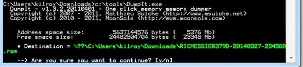
The first tool we need to make use of is the DumpIt tool. The DumpIt tool overcomes a challenge that we have. The challenge is that we shouldn’t be able to get direct access to memory. Memory should be managed by the operating system and we shouldn’t get direct access to it. This is especially true when it comes to writing to memory because you can cause problems if you somehow manage to sidestep the operating system and write directly to memory, you could overwrite critical operating system components or other programs that are executing and cause application of system crashes. It would be nice to keep all of our problems to a minimum and rather than diving into a lecture on the usefulness of separating functions into different rings where ring 0 has the highest level of privileges, we’ll just stick with getting our hands on some memory. We will use the DumpIt program to do that. Fortunately, it’s incredibly easy to use as you can see below. 

 

It’s really as simple as running DumpIt and then saying that you really want to continue when it asks you. You will then get a really large file that could be really, really large if you happen to have the kind of system that supports a LOT of memory. I’d say if you were the type of person who had a lot of money and could afford a lot of memory except that the price of RAM is supposed to be dropping, right? Well, at the very least it’s a lot easier and less expensive to get a metric buttload of memory now as compared with, say, the early 80s. Be aware that you need to make sure you have the disk space available to store the contents of your memory. If you have 4 gigabytes worth of memory on your system, you need at least 4 gigabytes of memory available to write to on your disk. 16G, 32G, whatever you have, make sure you have the disk space to store it because it’s all coming down. 

Once we have the memory capture from our running system, you should keep one thing in mind. Whatever else you get from the memory capture, you will definitely get artifacts from your use of DumpIt. In order to get the memory, DumpIt has to execute and in order to execute, it has to be in memory and if it’s in memory, it’s going to show up in the memory dump you are getting. Something to keep in mind. When you run a process list, you’ll see DumpIt in your process list. 

Now that we have a dump of memory, we need a good way of taking a look at it. As much fun as hex editors are, I find it’s difficult to find much of anything in a very large block of memory in a hex editor. We need a utility to automate the process. A utility that understands how memory is structure. A utility that knows where all the skeletons are buried, so to speak. We need Volatility. The Volatility Framework is a way of grabbing a lot of artifacts from a memory capture. In order to do this, though, it needs to know what type of memory capture we have. It uses a set of profiles in order to know what the memory layout looks like and where the different important structures are. We can determine the profile that is in use by using the command volatility imageinfo -f imagename.raw. You can see the output of that below, though I have substituted imagename.raw for the actual name of the image I got. I’m doing the analysis on a 64-bit Windows 7 Pro system, though the memory was captured from a Windows XP Pro system. 

 

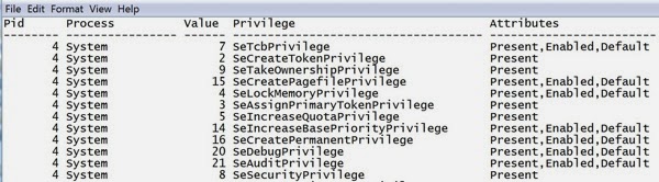
Once we have determined the profile, we can make any additional work much faster by providing the profile to volatility. As an example, we can get a list of the process privileges by using the priv command against our captured memory. This will present a list of the processes that were running when the capture took place and the privileges that are associated with it. In order to get that and also provide the profile, we can run volatility privs —profile=WinXPSP3x86 -f imagename.raw and it will skim through the memory dump, gathering all of that information. One of the problems we have is a limitation of the Windows command prompt and how Microsoft by default only allows 80 characters for the width of the window. You can increase the width, but it requires going into the properties and then dragging the window open. You can’t just drag the window open in Windows 7 and have the window adapt to the new size. Volatility, however, outputs in tables wider than 80 characters so your output will be wrapped, making it harder to read. We can write the output of any command to a text file by using —output-file=filename. You’ll get a text file with all of the relevant details. An example is the data below.

This output has been truncated in order to better fit in this page. There is, in actuality, a whole other column with a description field that has a text description of the privilege.

While we have done a couple of things to gather information, there is so much more to do but there isn’t as much point in walking through every single command available in Volatility when you can just go get yourself a copy of Volatility and play. Volatility has a number of Windows profiles and the default set of commands is targeted at the Windows profile. However, there are ways to analyze Linux memory captures and capturing Linux memory has its own unique set of challenges. That, however, is another task for another day.